Air Cargo Load Optimization using Quantum Annealing on Amazon Braket

by Rafael Sotelo, Laura Gatti, Juan Diego Orihuela, Rodrigo Acosta and Martin Machin

The cargo problem

A frequent problem amongst various transportation companies is determining the optimal loading strategy for packing their merchandise in different vehicles, such as boats, aircrafts, trains, or trucks. The case of air cargo exhibits particular characteristics that make the task especially difficult.  For example, the fuselage of the aircraft has a circular cross-section, which forces the unit load devices (ULDs) to have specific shapes to maximize the space utilized.

All cargo that is transported by aircraft must be consolidated in ULDs, i.e. it must be accommodated in containers and pallets of specific dimensions. There are different types of ULDs possible but these are standardized. Each ULD has a number of attributes:

• A weight associated w_i.

• Width and Length dimensions d_i, l_i respectively.

• An associated revenue v_i.

• A unique identifier of the package type Id_i

• A flag named type who indicates whether the container can go side by side or can only go in a single row.

The main problem of air cargo is to identify the optimal selection of the ULDs to be transported that maximizes the revenue transported in each aircraft, to a set of restrictions given by the physical constraints of the aircraft itself:

1. Weight restriction: Each deck supports a maximum weight that must be respected.

2. Volume restriction: There is a maximum volume of ULDs that can be transported on each deck.

3. Aftbay restriction: At the tail of the aircraft, on the main deck, there is an area which, due to the width reduction of the fuselage, it is impossible to fit side by side ULDs.

4. Center of gravity: The center of gravity of the load carried on the aircraft has to be within a specific range with respect to a target point on the length of the aircraft, in order to make the flight safe and to minimize fuel consumption.

5. Shear force restriction: In the same way, the load must be distributed in such a way that it respects the maximum shear force curve given by the manufacturer. Shear force is caused by the weight of the ULDs. To calculate the shear force the plane is modeled as two cantilevered beams supported at the center of the main deck. The lower decks are supported by these same beams, this means that the shear force from the lower decks can be simply summed.

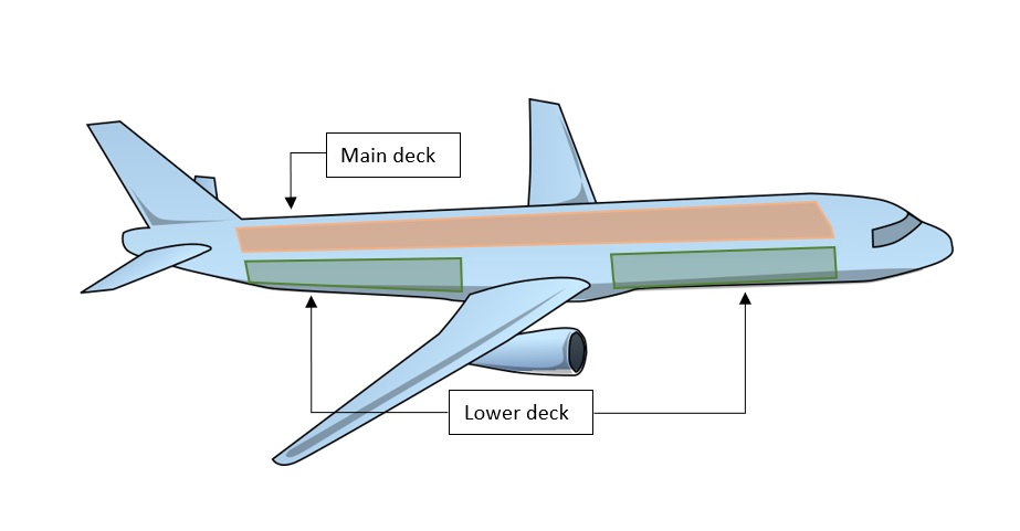
Depending on the aircraft, the warehouse area can be distributed between one, two or more cargo decks. A typical case is to have an upper deck and a lower cargo deck separated in two by a useless cargo area where the landing gear is located, for example.

Solution characteristics

Given a set of ULDs (N in total), which in general exceeds the capacity of the aircraft, the solution to the problem is to select a subset of these ULDs and give a specific position within the aircraft to each one, such that it maximizes the total associated revenue and satisfies the physical constraints of the aircraft.

Due to the exponential increase in the number of possible combinations as N increases, the problem poses a serious challenge to be solved by classical means. Some approaches include greedy algorithms, branch-and-bound, dynamic programming by weights or by profits, and also genetic algorithms and neural networks.

When using dynamic programming by weights, a series of problems for capacity values d = 0, . . . , c, computes profit values z_j(d). Then a certain recursion is applied for j = 1 up to j = n, yielding the optimum solution value as z_n(c). For example, the all-capacities knapsack problem is solved in this procedure, returning the optimal profit value z^∗ but not explicitly the optimal solution set of items, and the running time is O(nc).

It is in examples like this that quantum computing offers new possibilities for tackling these problems.  To model this problem in a way that a quantum computer can solve it is necessary to associate each possible charge configuration with a value, which can be interpreted as an energy. Therefore, the technique is to encode all possible configurations in a Hamiltonian that will be given to an annealing that will be able to find the lowest energy value. The better the charge configuration the lower should be its associated energy.

A toy example

In a very simplified case the selection problem bears great similarities to the classical NP-complete knapsack problem. Each unit of load stored in the warehouse is represented by binary variable xi ∈ {0,1} ∀i | 0 ≤ i ≤ N-1; with attributes revenue r_i, weight w_i, large l_i, unique number identification Id_i and a flag associated t_i.

For example, emulating the knapsack problem we can maximize revenue while the constraint could be total weight or volume occupied:

where C_max is the weight limit.

One way to translate this problem to a Hamiltonian is to use the formulation QUBO (quadratic unconstrained binary optimization). The most challenging part of this is transform the constraints into equalities in a way that they function as penalties. In the case of the knapsack constraint problem described above this can be done by taking the equality:

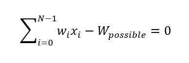
where ∑_(i=0)^(N-1)▒〖w_i x_i 〗 represents the total weight of the chosen configuration and W_possible the valid weights i.e. W_possible=0,1,2,… ,C_max . To express this as a quadratic formulation we must make use of auxiliary binaries variables y_j :

The second summation is the quasi-binary[1] representation of CMD where M = ⌊ log_2 (C_max) ⌋ and M+1 is the number of binary variables required for the representation and fulfills the role of  W_possible.  When the restriction is violated (the configuration exceeds C_max), the variables y_j will not be able to cancel the total weight and a positive energy will be added to this configuration.

Therefore, the total Hamiltonian of this toy model will have two parts, one for the optimization part and the other for the restriction part

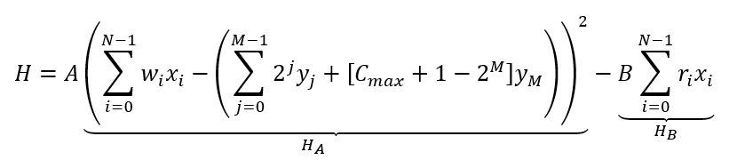
The term H_B is responsible for the maximization of the actual value put in the sack, and it is always less than or equal to zero (a maximization of positive numbers is switched for a minimization of negative numbers). The term H_A is a penalty when the restriction is violated, it is always positive except when it is canceled. The constants A and B are used to adjust scale differences between the variables value and weight and give the desired magnitude to each of the components. E.g if A is too small, in terms of energy, it may be better to add an element of great value even if it violates the weight restriction since the penalty is less than the negative energy gain by H_B

The real solution

As can be deduced the previous part is a much easier version of the general problem. Each of the constraints posed in the problem description must be modeled and added to the Hamiltonian.

In fact, the weight constraint shown here is the easiest of all. For example, in the volume constraint must consider that not just any type of ULDs can go anywhere in the airplane. Very tall ULDs cannot be placed sideways, or very wide ULDs cannot be placed in the tail of the airplane (Aftbay restriction).

And there is not only the problem of selection, but there must also be the way in which these ULDs are ordered inside the plane in such a way that they comply with the center of gravity and shear force restrictions.

In total, a complete version that meets the requirements explained in the first part can be obtained using two QUBOS with multiples adding each one:

Each Boolean variable needs at least one qubit for its representation as a state variable in a quantum computer. An estimate of the total number of qubits required depends on the physical parameters of the plane and the characteristics of the set of ULDs to be loaded:

• N is the number of container available.
• C_MD is the maximum load bearing weight of the main deck.
• 〖l_MD〗_max is the maximum length of the cargo bay.
• AB is the length of the aft part of the bay where only type 2 ULDs can be placed.
• Q is the smallest number to represent the maximum number of ULDs in side-by-side position entering the aircraft

An upper bound of the number of qubits required may be to implement the QUBO H_M is given by

Qubits requirement = 2N +M+R+K+Q+3

Where M = ⌊log_2⁡(C_MD ) ⌋ ,R=⌊log_2 (2〖l_MD〗_max )⌋ , K=⌊log_2 (AB)⌋

The number of qubits required by I_M is significantly less.

[1] The quasi binary representation of a number  is obtained by taking M+1 boolean variables y_k with M = ⌊ log_2 (c) ⌋ for its binary expansion in which the coeficient of the most significant term y_M is changed from  2^M to (c + 1-2^M) . Therefore, the range of values that can be represented with the Boolean variables goes from 0 to c . In this representation values smaller than c can have more than one valid configuration.

Example of the problem

We run our algorithm adjusted to the physical characteristics of the A330 200F aircraft[1]. The Airbus 330 200F is an aircraft specially designed for cargo operations. It consists of a main deck and two lower decks plus a bulk cargo loading space.

---

[1] https://aircraft.airbus.com/en/aircraft/freighters/a330-200f

Two sets of 220 randomly generated ULDs are given as input, one for the main deck and the other for the lower deck. They must be in csv file with the format:

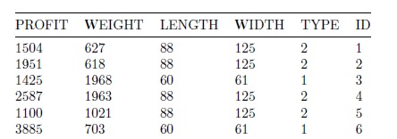
Weight, length and width must match the dimensions of some of the standardized ULDs compatible with the A330 200F specifications.

The algorithm takes as maximum load parameters:

• Main deck available length: 1540
• Main deck max. weight: 40000
• Lower decks available length: 866
• Lower decks max. weight: 20000
• We have modeled the airframe as two cantilevered beams, supported in the middle point between the wings.
• The center of gravity is targeted in the middle point between the wings.

The output of our algorithm is a possible configuration of the load inside the aircraft:

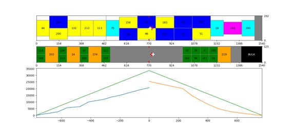
The upper graph contains the exact position of each selected ULD in the aircraft. Both on the main deck and on the lower deck. The gray spaces are unused volumes. In the case of the lower deck the space between decks is due to structural characteristics of the aircraft and must be left empty.

The lower graph shows the aircraft load distribution. The light blue and orange graphs show the shape of the shear curve for the ordering of ULDs shown in the upper graph. The green lines are the extreme shear curve that is taken for the aircraft and should not be exceeded. It was calculated assuming the maximum weight uniformly distributed loads along the decks.

Each color corresponds to a standardized ULD type. In this example the yellow-colored containers are placed both side by side and in a single row.

It can also be seen that the solution leaves available volume in both the main deck and the lower deck before the bulk. This is because the objective to optimize is revenue. In this case it may be convenient to waste some space but carry the most valuable ULDs. It should be noted that the excess space does not fit more ULDs. The same could be true for the total weight carried. Our algorithm can be set in such a way that the total load carried can be prioritized to complete the possible weight of the aircraft or its volume. In the following example we compare the result we would get from prioritizing volume over load:

---

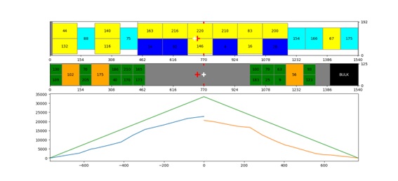
An intermediate result would be obtained by balancing the counters:

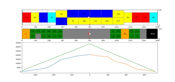
Finally, it is possible to compare these three results in a single graph, considering the main performance factors of the three configurations.

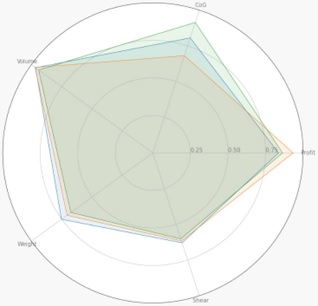
• CoG (Center of Gravity) indicator refers to the exactitude of the solution with respect to the CoG objective, where 1 indicates no deviation and 0 represents 25 or more inches.
• Profit indicator is the profit of the solution as a percentage of an arbitrary number, 110.000 in this case.
• The Shear indicator measures mechanical stress on the airframe, a larger number means more stress.
• The weight indicator is the loaded weight as a percentage of the maximum allowable
• The volume indicator is the filled volume as a percentage of the available volume

Running on Amazon Bracket and D-Wave

First, we need to set up the environment and create a Notebook Instance.

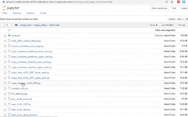
With the Jupyter notebook created, we will work on Python code for our algorithm:

We have a group of files, including source code, data, and configuration.

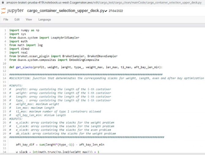
We have our main application code,

and the area where we set up the D-Wave configuration using the LeadHybridSampler. In D-Wave environment a sampler accepts a problem in binary quadratic model (BQM) or discrete quadratic model (DQM) format and returns variable assignments. Samplers generally try to find minimizing values but can also sample from distributions defined by the problem. The LeadHybridSampler is a class for using Leap’s cloud-based hybrid BQM solvers. Leap’s quantum-classical hybrid BQM solvers are intended to solve arbitrary application problems formulated as binary quadratic models (BQM). You can configure your solver selection and usage by setting parameters, hierarchically, in a configuration file, as environment variables, or explicitly as input arguments.

Then we use the Amazon Braket Ocean Python Plugin which is an open-source library in Python that provides a framework that you can use to interact with Ocean tools on top of Amazon Braket. We have a class for using DWave-formatted parameters and properties with Amazon Braket as a sampler (BraketSampler and BraketDWaveSampler).

There are dimod composites that provide layers of pre- and post-processing (e.g., minor-embedding) when using the D-Wave system. We use the EmbeddingComposite: it maps problems to a structured sampler. Automatically minor-embeds a problem into a structured sampler such as a D-Wave system. A new minor-embedding is calculated each time one of its sampling methods is called.

In the environment we have several D-Wave machines:

And from the code we select which one we will connect to, using the corresponding functions.

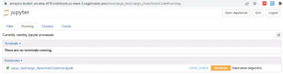
Once we run the code, we can monitor the execution in the console:

We have our initial input data shown before the quantum algorithm is called, while we wait for the result:

As a result, we will get a structured data with the solution parameters:

We create a json structure with the data and provide a printed solution:

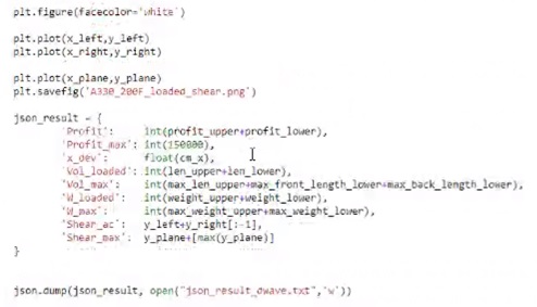
The diagram shows the location of the ULDs and how the shrear limits are met.

This quantum application can solve the load of ULDs into full freighters configurations like Airbus A330-200F and Boeing 747-400 and larger aircrafts. This solution is ready to run proofs of concept today.